Overview
Chombo needs to operate in a non-rectangular domain for three potential applications:
- Toroidal MHD application with PPPL: In this application the grid needs to be non-rectangular in physical space. The high degree of anisotropy for the diffusion of electrons makes it necessary to align the constant-jk grid lines with the magnetic field. This requires a singularly-periodic Cartesian rectangular domain to be mapped into a field-conforming toroidal physical space.
- Earth atmosphere simulation: This application requires a 3D grid as a shell over a spherical surface. A single rectangle cannot map to the surface of a sphere without polar singularities and sub-optimal grid concentration at the poles (for example, a Mercator projection). An alternative is to use a cubic (or other rectangular-faced solid such as an icosahedral) and a Gnomonic projection. This requires a multi-block Cartesian space with non-trival connectivity and mapped blocks.
- Edge plasma simulation: As in the MHD application, coordinates defined by the magnetic field are advantageous. The ``single null'' topology of an edge plasma in any poloidal plane can be mapped to eight rectangular subdomains that all connect at a single point on the sparatrix. In addition, the desire for near-magnetic-field-aligned coordinates and the potential for large distortion of cells with toriodal progression make a mapped multi-block mesh decomposition in the toroidal direction attractive as well.
In the mapped multi-block framework, computations are on a set of separate blocks, on each of which we specify:
- a rectangular region in mapped space, called the domain of the block;
- a continuous and one-to-one mapping function, having an inverse that is also continuous and one-to-one; and
- a region in real space, called the range of the block, that is the range of the mapping function applied to the domain of the block in mapped space.
Blocks must satisfy the following requirements:
- In mapped space, the domains of different blocks must be disjoint.
- In real space, the ranges of different blocks may intersect only at their boundaries.
As in the rest of Chombo, data are held on rectangular patches. In the mapped multi-block framework, each patch must be contained in only one block. In other words, no patch may straddle two or more blocks.
Examples
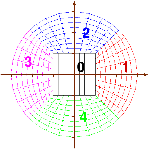
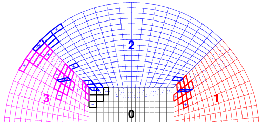
Domain in 2D mapped space: five squares Range in 2D real space: disk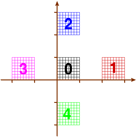
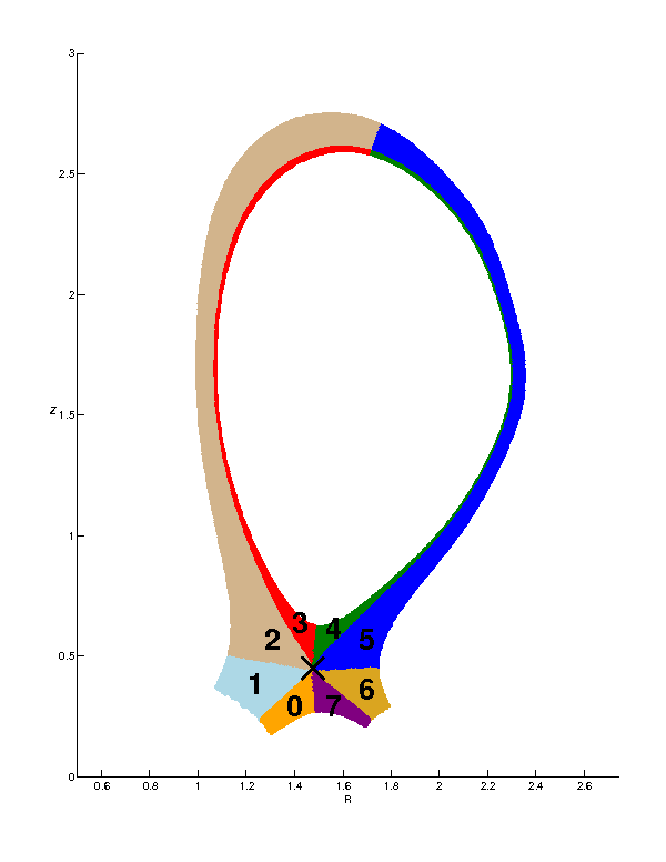
Domain in 2D mapped space: eight squares Range in 2D real space: single-null edge plasma geometry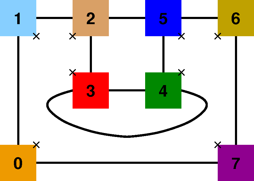
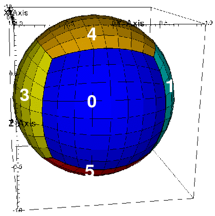
Domain in 2D mapped space: six squares Range in 3D real space: surface of sphere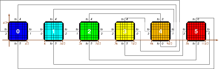
Advection on a sphere, with one level of refinement
Exchanging data between blocks
Exchange operations in Chombo fill in ghost cells of a patch using data from other patches. A ghost cell of a patch is always outside the patch, but in the mapped multi-block framework, the ghost cell may be inside or outside the block containing the patch. If the ghost cell is inside the same block that contains the patch, then it can be filled simply by copying its data. But if the ghost cell lies outside the block containing the patch, the exchange operation is more complicated, and in this case the ghost cell must be filled by interpolation.
The ghost cells of a patch that lie outside the block containing the patch will be called extra-block ghost cells of the patch. Two layers of extra-block ghost cells of block 2 of the disk example are outlined with dotted blue lines below, in both mapped space and real space. The centers of four of them are marked with blue *. The cells of the interpolation stencils of these four ghost cells are shown with thicker outlines, each with the color of its block.
In mapped space: four ghost cells with their interpolation stencils In real space: four ghost cells with their interpolation stencils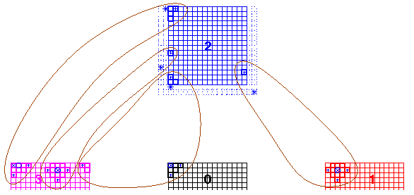
The function value for each extra-block ghost cell is interpolated from function values for the valid cells in its stencil.
Around each ghost cell, we approximate the function by a Taylor polynomial in real coordinates, of degree P. This polynomial has different coefficients for each ghost cell. In 2D the polynomial is of the form:
where (Xg, Yg) is the center of the ghost cell in real coordinates, and R is the mean distance from (Xg, Yg) to the centers in real space of the stencil cells of g.
Starting with averaged values of f over each valid cell, then the coefficients apq come from solving the overdetermined system of equations
where there is an equation for every cell j in the selected neighborhood of valid cells of the ghost cell. The notation
indicates an average over cell j.
The average value of f on the ghost cell is then obtained by
.